This Package estimates a Vector Autoregressive Model with an External Instrument in R. It is based on

“Inference in Structural Vector Autoregressions Identified With and External Instrument”, Montiel Olea, José L; Stock, James H.; and Watson, Mark W; Working Paper Columbia University. Link

The corresponding Matlab code and sample data can be found here: https://github.com/jm4474/SVARIV

Installation:

install.packages(“devtools”) devtools::install_github(“https://github.com/martinbaumgaertner/varexternal.git”) library(varexternal)

Content

For now two different Confidence Intervals (CI) for Impulse responses are included:

1. Delta Method

2. Anderson-Rubin confidence set

   The confidence interval is robust to the construction of weak-instrument. Note that for strong instrument estimation the CI convergence to standard CI intervals.

In addition the authors propose an modified Wald test as a test for weak instruments concerns which is also included in the package. Bootstrap procedures are currently not included.

[…] these weak instrument robust confidence sets should routinely be used for impulse response coefficients identified with an external instrument. Along with our weak-instrument robust confidence sets, we suggest that practitioners report either the Wald statistic for the null hypothesis that the external instrument is irrelevant, or the heteroskedasticity-robust first-stage F-statistic as described in Section 4.2. Large values of these statistics(e.g., above >10) suggest approximately valid coverage of standard 95% confidence intervals.” (Olea, Stock, Watson 2018)

Disclaimer: Although the methodology and the basic code is not mine, all errors are first to be credited to me personally. Please note that this package has not yet been tested extensively. I am grateful for every hint for improvement.

Example

#load package
library(devtools)
install_github("martinbaumgaertner/varexternal")
library(varexternal)

    data(oil)

    ydata<-oil[,1:3]
    z<-oil[,4]
    p           = 24    #Number of lags in the VAR model
    NWlags      = 0;  # Newey-West lags(if it is neccessary to account for time series autocorrelation)
    norm        = 1; # Variable used for normalization
    scale       = 1; # Scale of the shock
    horizons    = 20; #Number of horizons for the Impulse Response Functions(IRFs)
    confidence=c(0.6,0.9,0.95);

    VAR<-SVARIV(ydata,z,p,confidence,NWlags,norm,scale,horizons,instrument_name="test")

    sh.col<-      c("#E41A1C")
    names(sh.col)<-c("test")
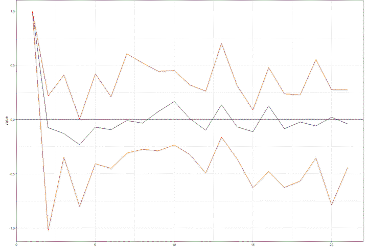
    pretty_irf(data=list(VAR$irfs),shock_names="test",pretty_names=c("a","b","c"),manual_color=sh.col,title="subheading")